
Integrated Computational Materials Engineering (ICME)
Multiscale Study of Pure Chromium
Abstract
In this work, we apply multiscale modeling techniques associated with
Integrated Computational Materials Engineering (ICME) in order to capture the
plastic behavior of pure chromium (Cr). We used Density Functional Theory (DFT)
in the open-source software Quantum Espresso (QE) to generate energy versus
volume (EV), energy versus atomic separation (EA), and generalized stacking
fault energy (GSFE) curves along with the lattice parameter, bulk modulus, and
cohesive energy at equilibrium. The Modified Embedded Atom Method (MEAM)
Parameter Calibration tool along with the DFT data was utilized to create a
MEAM potential for Cr. Both sets of simulations were verified by comparison to
values from literature, and a sensitivity analysis was conducted for the MEAM
potential. These lower scale simulations are upscaled to Dislocation Dynamics
(DD) computations. Information is bridged from atomistics to the microscale by
tracking dislocation mobility and quantifying the stress-strain behavior. A
convergence study is conducted on different sized crystal structures and
dislocation mobility calculations with the Large-scale Atomic/Molecular
Massively Parallel Simulator (LAMMPS) program. The mobility is calculated from
seven simulations at varying applied shear stresses from 250 MPa to 3000 MPa,
or 2500 to 30000 bar, respectively. These calculations were run with three sets
of MEAM parameters to find an upper and lower bound for our data. The
post-processing program OVITO was used to visualize the centrosymmetry
parameter, thermal equilibrium, and track dislocation mobility. Then, we
generated position versus time plots for each simulation to calculate the
dislocation velocity, dislocation mobility, and drag coefficient. Three sets of
stress-strain curves were found from a single Frank-Read source in Multiscale
Dislocation Dynamics Plasticity (MDDP) computations.
Keywords: Chromium (Cr), Modified Embedded Atom Method (MEAM), Density
Functional Theory (DFT), Integrated Computational Materials Engineering (ICME),
Generalized Stacking Fault Energy (GSFE), Molecular Dynamics (MD), Dislocation
Dynamics (DD), Large-scale Atomic/Molecular Massively Parallel Simulator
(LAMMPS), Multiscale Dislocation Dynamics Plasticity (MDDP)
Author(s): Cagle, M. S., Fonville, T. R., Kazandjian, S. L., and Sprow, B. T.
Introduction
Horstemeyer [1] proposed the ICME paradigm as a means to capture the multi-scale phenomenon of a material by bridging information between length scales from the electron scale to the structural (continuum) scale. Multiscale modeling with the ICME paradigm offers the accuracy required to predict failure, reduce design costs, and reduce time-to-market with the simulation-based design paradigm. The fundamental steps required to achieve multiscale modeling with the ICME paradigm are as follows:- Step 1: Downscaling, where we define the desired higher-level “effects,” or information needed.
- Step 2: Modeling and simulation at lower length scales (including calibration and verification)
- Step 3: Upscaling, where we pass information up to meet the requirements set at the higher length scale in step 1. Iteration is required to ensure a proper connection.
- Step 4: Validation at the higher length scale through experiment or simulation.
According to the ICME methodology [3], capturing plastic deformation of Cr at the macroscale requires the linking of atomistic and DD simulations at lower length scales. A convergence study is performed to determine the appropriate atomic size for our DD simulations using the calibrated MEAM potential and an applied shear stress of 1500 MPa (15000 bar). Then, we vary the MEAM potential to create an upper and lower bound. We used the three MEAM potentials to run Molecular Dynamics (MD) simulations within the LAMMPS program. Seven simulations were performed per MEAM potential with an applied shear stress ranging from 250 to 3000 MPa (2500 to 30000 bar). We visualized the simulation results with the open-source visualization tool “Ovito.” In Ovito, we can study the centrosymmetry parameter, crystal structures, thermal equilibrium, and dislocation behavior. The dislocation behavior was captured and used to create position vs. time plots that we use to calculate dislocation velocity and dislocation mobility. The dislocation mobility was then passed on to run MDDP calculations. We can use the MDDP calculations with a single Frank-Read source to describe the stress-strain behavior. Three stress-strain curves are generated from the MDDP calculations utilizing the three MEAM parameters used to calculate an upper and lower bound for the dislocation mobility.
Materials and Methods
Density Functional Theory (DFT)
Energy vs. Volume (E-V) Curve
We plotted initial energy versus lattice parameter (E-A) and energy versus volume (E-V) curves from points calculated with Quantum Espresso (QE). The range of values was 80 – 120% of the assumed lattice constant of chromium (2.880). We set the initial K-point grid to 3 and assumed a constant energy cutoff value of 30 Rydberg. We show the initial E-A and E-V curves below in Figures 1 and 2, respectively.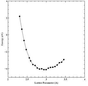
Figure 1. Initial Energy (eV) versus lattice parameter (A) curve for BCC chromium.
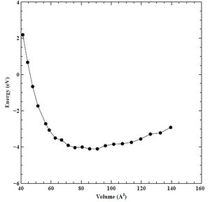
Figure 2. Initial Energy (eV) versus Volume (V) curve for BCC chromium.
KPOINT Convergence
Next, we performed a convergence study on a single atom of BCC chromium to determine which K-point grid offered a good tradeoff between lattice parameter, bulk modulus, minimum cohesive energy, and CPU time. We varied the K-points from 1 to 10 and plotted the results against derived parameters. We held energy cutoff constant at 30 Rydberg through each K-point convergence study. We show the K-point versus lattice parameter, bulk modulus, minimum cohesive energy, and CPU time plots below in Figures 3-6. We determine a K-point grid of 16 constituted convergence of lattice parameter (± 0.00086 A), bulk modulus (± 1.963958 Kbar), and minimum cohesive energy (± 0.000753 eV) without requiring more CPU time. Using our converged K-point grid, we conducted a second convergence study on a single atom of BCC chromium to determine which energy cutoff value offered a good tradeoff between lattice parameter, bulk modulus, and CPU time. We varied the energy cutoff values from 20 to 100 Rydberg and then plotted the results against the derived parameters. We show the energy cutoff versus lattice parameter, bulk modulus, minimum cohesive energy, and CPU time plots below in Figures 7-10.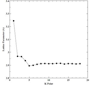
Figure 3. Lattice parameter versus K-point grid for BCC chromium.
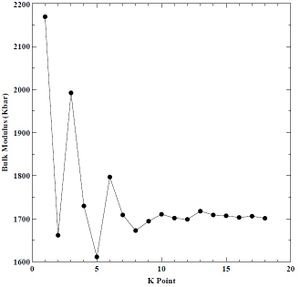
Figure 4. Bulk modulus versus K-point grid for BCC chromium.
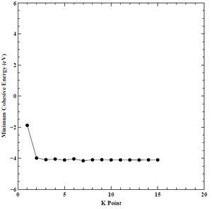
Figure 5. Minimum cohesive energy versus K-point grid for BCC chromium.

Figure 6. CPU time versus K point grid for BCC chromium.
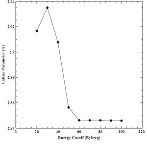
Figure 7. Lattice parameter versus energy cutoff for BCC chromium.
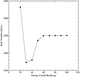
Figure 8. Bulk modulus versus energy cutoff for BCC chromium.
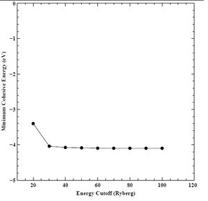
Figure 9. Minimum cohesive energy versus energy cutoff for BCC chromium.
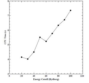
Figure 10. CPU time versus energy cutoff for BCC chromium.
Equation of State (EOS)
We determined an energy cutoff of 60 Rydberg constituted convergence of lattice parameter (± 0.000144 A), bulk modulus (± 1.623263 Kbar), and minimum cohesive energy (± 0.000896 eV) without requiring more CPU time. Next, we compared two equations of state (EOS), namely, Birch and Murnaghan. We use an EOS to derive the lattice parameter, bulk modulus, and minimum cohesive energy. We show the results for lattice parameter, bulk modulus, and minimum cohesive energy using the Birch EOS below in Figures 11-13. We do not find good convergence for our lattice parameter, bulk modulus, or minimum cohesive energy using the Birch EOS. We show the results for lattice parameter, bulk modulus, and minimum cohesive energy using the Murnaghan EOS below in Figures 14-16. Again, we do not find good convergence for our lattice parameter, bulk modulus, or minimum cohesive energy using the Murnaghan EOS. However, we select the Birch EOS for because the results for the three parameters were closer to experimental values found in the literature.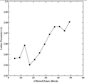
Figure 11. Lattice parameter versus number of plotted points for BCC chromium with the Birch equation of state.
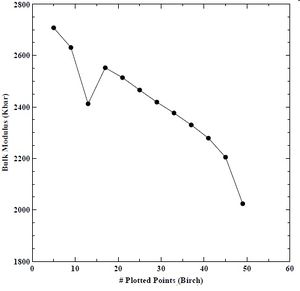
Figure 12. Bulk modulus verses number of plotted points for BCC chromium with the Birch equation of state.
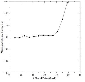
Figure 13. Minimum cohesive energy versus number of plotted points for BCC chromium with the Birch equation of state.
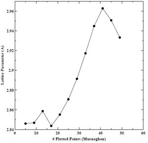
Figure 14. Lattice parameter versus number of plotted points for BCC chromium with the Murnaghan equation of state.
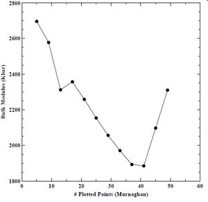
Figure 15. Bulk modulus verses number of plotted points for BCC chromium with the Murnaghan equation of state.
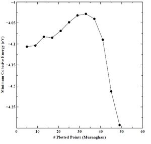
Figure 16. Minimum cohesive energy versus number of plotted points for BCC chromium with the Murnaghan equation of state.
Final Converged E-A and E-V Plots
Finally, using our converged K-point grid (16 points), and converged energy cutoff (60 Rydberg) values, we created a set of energy versus lattice parameter (E-A) and energy versus volume (E-V) curves for the primary chromium crystal structure (BCC), as well as the secondary (FCC) and tertiary (HCP) crystal structures. We show the final E-A and E-V curves for BCC, FCC, and HCP chromium below in Figures 17-22.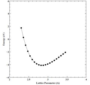
Figure 17. Converged energy versus lattice parameter (E-A) plot for BCC chromium.

Figure 18. Converged energy versus volume (E-V) plot for BCC chromium.
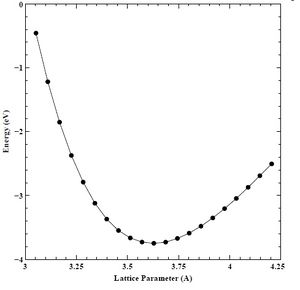
Figure 19. Converged energy versus lattice parameter (E-A) plot for FCC chromium.
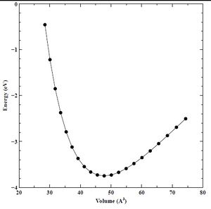
Figure 20. Converged energy versus volume (E-V) plot for FCC chromium.
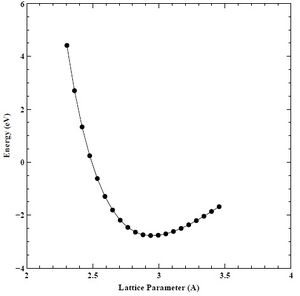
Figure 21. Converged energy versus lattice parameter (E-A) plot for HCP chromium.
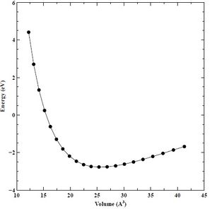
Figure 22. Converged energy versus volume (E-V) plot for HCP chromium.
Generalized Stacking Fault Energy (GSFE) Curves
We ran DFT simulations in QE to generate the GSFE curves for pure chromium using a Python script available here. This script can generate GSFE curves along the three BCC slip systems presented in Table 1.Table 1: Input Parameters for GSFE Curve Python Script
| Name | Slip Plane | Slip Direction |
|---|---|---|
| Full | (110) | [-111] |
| Partial | (110) | [001] |
| Longpartial | (110) | [-110] |
Table 2: Input Parameters for GSFE Curve Python Script
| Parameter | Value |
|---|---|
| Lattice Parameter | 2.8497783 Å |
| Energy Cutoff | 60 Ry |
| Number of K-points | 16 |
| Element Weight | 51.9961 atomic units[4] |
| Smear | 0.06 |
| Vacuum Size | 20.0 |
| Number of Stacking Layers | 10 |
GSFE Curves
We generated GSFE curves for pure chromium along three BCC slip systems: (110)[-111] (full), (110)[001] (partial), and (110) [-110] (longpartial). We computed sixteen GSFE data points for all three slip systems. Data for the longpartial slip system only spanned half of the slip distance; therefore, we assumed this curve was symmetric based on the symmetry of the BCC structure. We show the GSFE curves (change in energy versus upper atom displacement) in Figure 23 below. The Y-axis represents change in energy (mJ/m²), and the X-axis represents displacement normalized by lattice parameter (2.8497783 Å).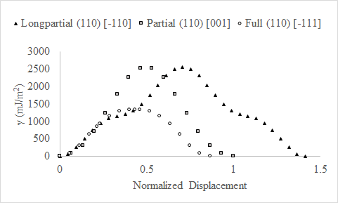
Figure 23. Change in stacking fault energy (γ) versus displacement normalized by lattice parameter (2.8497783 Å) for the longpartial and full slip systems.
In Figure 24, we compare data from our full slip system GSFE curve with DFT from Yang et al. [5]. The axes in Figure 24 are the same as in Figure 23 except both curves are scaled such that the displacement spans zero to one. Our DFT calculations show close agreement with Yang et al.[5].
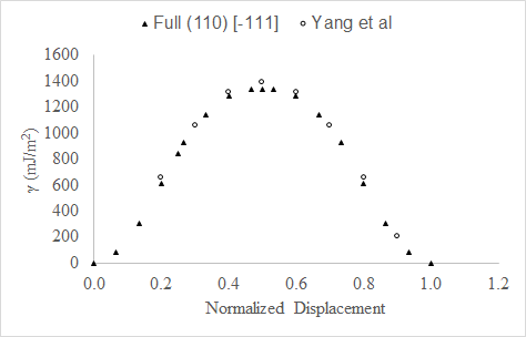
Figure 24. GSFE curves from this study and DFT calculations from Yang et al. [5] along the full slip system show close agreement. Both curves are scaled such that displacement spans zero to 1.
Modified Embedded Atom Method Potential Calibration
MEAM potential calibration has been a manual process since the creation of the MEAM model. Horstemeyer et al.[2] presented a simple MEAM potential calibration methodology with the MPC software tool. In this work, we follow a similar approach where we calibrated BCC, FCC, and HCP energy versus lattice spacing using energy versus atomic volume (E-V) data produced in QE. After loading the E-V curve results from DFT, we calibrate the MEAM model parameter values of equilibrium lattice constant (alat), energy per unit volume (esub), and the constant related to the bulk modulus (alpha) for LAMMPS to match the minimum BCC energy as shown in Figure 25 below.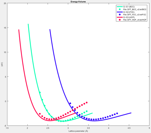
Figure 25. BCC, FCC, and HCP E-V curves after calibration to DFT data.
Sensitivity Analysis
We calculate values far away from equilibrium using the attract and repuls parameters proposed by Hughes et al.[6] that represent the cubic attraction and repulsion terms in the UEOS. We use single crystal elastic moduli experimental values from Yang et al.[5] (Table 3) to calibrate the MEAM potential elastic constants by varying the screening parameter, Cmin, scaling factor for embedding energy, asub, and exponential decay factor for atomic density, b0. These variables were shown to have the largest effect on the E-V curve calibration based on parametric sensitivity studies.Table 3: Comparison of experimental and MEAM single crystal chromium elastic stiffness constants (GPa)[5].
| Elastic Constant | Experimental | MEAM |
|---|---|---|
| C11 | 391.0 | 391.0 |
| C12 | 89.6 | 89.6 |
| C44 | 103.2 | 103.2 |
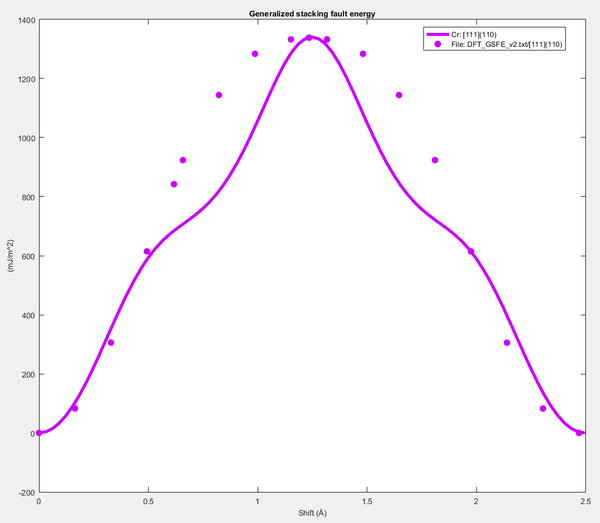
Figure 26. Calibrated GSFE versus shift plot.
Table 4: MEAM model parameter values after calibration to DFT simulation data.
| Name | Calibrated Value | Name | Calibrated Value |
|---|---|---|---|
| alat | 2.9891 | esub | 4.3477 |
| asub | 0.6146 | alpha | 5.5799 |
| b0 | 5.5535 | b1 | 1.0000 |
| b2 | 5.0000 | b3 | 1.0000 |
| t0 | 1.0000 | t1 | 1.0000 |
| t2 | 0.0000 | t3 | 10.6000 |
| Cmax | 2.5418 | Cmin | 0.9839 |
| attract | 0.0000 | repuls | 0.0000 |
Molecular Dynamics
Atomic Position Generation
We generated the atom positions files for dislocation mobility simulations via a Fortran routine available on Atomistic Dislocation Generation. To setup the code, we selected the body centered cubic (BCC) crystal structure to match the crystal structure of Cr. Then, we selected to study an edge dislocation for a Periodic Array of Dislocations (PAD). The atom positions application does not allow for custom lattice parameters with BCC crystal structures. For this reason, we selected the pre-programmed iron, which has the closest lattice parameter (2.85 Å) to chromium. However, the first step of each LAMMPS simulation equilibrates the system using the user-provided MEAM potential, which moves the atoms to the lowest energy state. This allows for a slight tolerance in the initial lattice parameter; simulations can be visually inspected after equilibrium to check that the initial lattice parameter does not adversely affect the resulting structure as was the case in our simulations.Dislocation Mobility
Dislocation Velocity vs. Applied Shear StressTo study the effect of number of atoms on dislocation mobility, we conducted six LAMMPS simulations with a constant applied shear stress of 1500 MPa (15000 bar). We varied the number of unit cells in the X and Y directions to produce the different volumes. We held the number of unit cells in Z constant at 3 unit cells because the edge dislocation is assumed to be infinitely long in this direction. Therefore, Z dimension can be accurately modeled with only a few unit cells. The number of unit cells in X and Y were selected and varied consistently to prevent edge and size effects. The X direction was the largest dimension because the dislocation translates in the X direction. In Table 5 below, we show the atom position sizes and their resulting dislocation velocity.
Table 5: Atom position convergence study parameters and results
| Simulation | (X, Y, Z) units | # of atoms | Velocity (nm/ps) |
|---|---|---|---|
| 1 | 11 x 10 x 3 | 330 | 0.416 |
| 2 | 31 x 14 x 3 | 1302 | 0.243 |
| 3 | 41 x 20 x 3 | 2460 | 0.133 |
| 4 | 55 x 36 x 3 | 5940 | 0.102 |
| 5 | 73 x 34 x 3 | 7446 | 0.104 |
| 6 | 97 x 46 x 3 | 13386 | 0.104 |
MEAM Parameter Bounds
Previously, we calibrated a MEAM parameter with respect to energy vs. lattice parameter, energy vs. volume, elastic constants, and the Generalized Stacking Fault Energy (GSFE) curve. In this section, we use the calibrated MEAM parameter as a mean value and generate a set of upper and lower parameters by varying the GSFE curve. We found the t3 parameter had the largest influence on the GSFE curve; therefore, we conducted a parametric study on this parameter to find a GSFE curve that has a peak value approximately 10% higher and lower than the mean. We show the parametric study and results from the MEAM Parameter Calibration (MPC) tool in Figure 27 below.
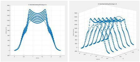
Figure 27. Parametric study on the Generalized Stacking Fault Energy Curve (GSFE) with the t3 parameter ranging from -1 to 1.
Dislocation Velocity vs. Applied Shear Stress
In this section we study the effect of applied shear stress on dislocation velocity for the three sets of MEAM parameters to determine the dislocation mobility. We conducted seven simulations for each MEAM parameter set to study the effect of applied shear stress on dislocation velocity. The applied shear stresses ranged from 250 MPa to 3000 MPa, or 2500 to 30000 bar, respectively. From the position vs. time results, we can calculate dislocation velocity as the slope of each line. Then we convert angstroms to nanometer by multiplying each result by 0.1. In Figure 28 below, we show the results for all 21 simulations velocity versus applied shear stress.
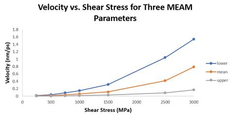
Figure 28. Velocity vs. shear stress for mean, upper, and lower MEAM parameters.
Table 6: Mobility and Peierls Stresses for three MEAM parameters.
| MEAM Parameter | Mobility (1/Pa*s) | Peierls Stress (MPa) | Drag Coefficient (Pa*s) |
|---|---|---|---|
| Lower | 726 | 204.34 | 0.00138 |
| Mean | 277 | 167.41 | 0.0036 |
| Upper | 70.7 | 174.82 | 0.0141 |
Dislocation Dynamics
MDDP with Single Frank-Read Source
We generated a single Frank Read Source (FRS) pair within BCC chromium using Multiscale Dislocation Dynamics Plasticity (MDDP). This software illustrates dislocation movement throughout a crystal. The input files included values shown in Table 7. Dislocation mobility was calculated from previous LAMMPS simulations for a lower, mean, and upper MEAM parameter set.Table 7: Chromium input parameters for MDDP.
| Parameter | Value |
|---|---|
| Crystal Size (Burger's vectors) | 10000 X 10000 X 10000 |
| X-direction | [1 0 0] |
| Y-direction | [0 1 0] |
| Z-direction | [0 0 1] |
| Strain Rate | 1e5 |
| Loading Direction | X-axis |
| Density (kg/m3) | 7190 |
| Shear Modulus (GPa) | 110 |
| Poisson’s Ratio | 0.31 |
| Burger’s Vector Length (m) | 2.47E-10 |
| Temperature (K) | 300 |
| Stacking Fault Energy (J/m2) | 1.338 |
| Lower Bound Dislocation Mobility (1/Pa*s) | 726 |
| Mean Dislocation Mobility (1/Pa*s) | 277 |
| Upper Bound Dislocation Mobility (1/Pa*s) | 70.7 |
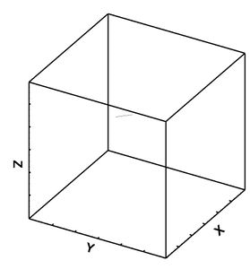
Figure 29: Initial state for lower bound.
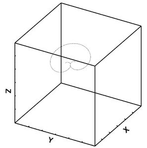
Figure 30: Dislocation movement for lower bound after 2 frames.

Figure 31: Dislocation movement for lower bound after 4 frames.
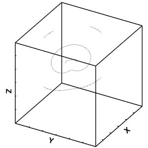
Figure 32: Dislocation movement for lower bound after 6 frames.
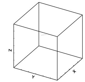
Figure 33: Initial state for mean.
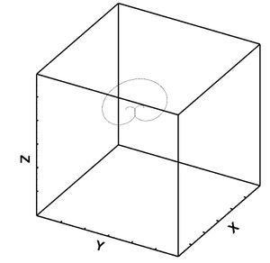
Figure 34: Dislocation movement for mean after 2 frames.
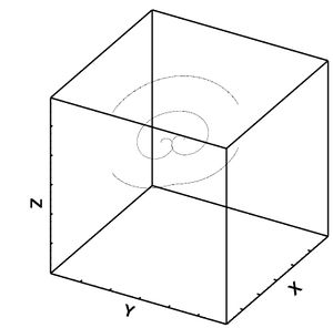
Figure 35: Dislocation movement for mean after 4 frames.
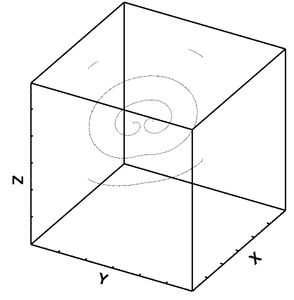
Figure 36: Dislocation movement for mean after 6 frames.
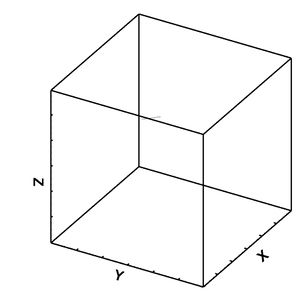
Figure 37: Initial state for lower bound
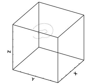
Figure 38: Dislocation movement for lower bound after 2 frames
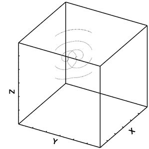
Figure 39: Dislocation movement for lower bound after 4 frames
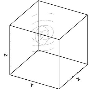
Figure 40: Dislocation movement for lower bound after 6 frames
MDDP with multiple Frank-Read Sources
We generated a multiple Frank Read Source (FRS) pairs within BCC chromium using Multiscale Dislocation Dynamics Plasticity (MDDP). This software illustrates dislocation movement throughout a crystal. The input files included values shown in Table 8. Dislocation mobility was calculated from previous LAMMPS simulations for a lower, mean, and upper MEAM parameter set.Table 8: Chromium input parameters for multiple Frank Read Sources in MDDP.
| Parameter | Value |
|---|---|
| Crystal Size (Burger's vectors) | 10000 X 10000 X 10000 |
| X-direction | [1 0 0] |
| Y-direction | [0 1 0] |
| Z-direction | [0 0 1] |
| Strain Rate | 1e5 |
| Loading Direction | X-axis |
| # Frank Read Source Pairs | 10 |
| Density (kg/m3) | 7190 |
| Shear Modulus (GPa) | 110 |
| Poisson’s Ratio | 0.31 |
| Burger’s Vector Length (m) | 2.47E-10 |
| Temperature (K) | 300 |
| Stacking Fault Energy (J/m2) | 1.338 |
| Lower Bound Dislocation Mobility (1/Pa*s) | 726 |
| Mean Dislocation Mobility (1/Pa*s) | 277 |
| Upper Bound Dislocation Mobility (1/Pa*s) | 70.7 |
Determination of Voce Hardening Law
We calculated the Voce hardening law parameters by using Equation 1[5].Where K is hardening, α is a constant relating to strength (assumed to be 0.35[4]), μ is the shear modulus (110 GPa for chromium), b is the Burger’s vector (2.47E-10 m for chromium), and ρ is the dislocation density. We determined dislocation densities from MDDP and plugged those values into Equation 1 to calculate kappa (κ). We plotted K values against time, and determined initial strength (κ0), saturation strength (κS), and initial hardening rate (h0) from the decaying exponential function (Equation 2[5]).
K0 is the starting value of kappa versus time, and Ks is the asymptotic value in which the function converges. The hardening rate (h0) is the fitted slope in Excel of the decaying exponential graph. Figures 41, 42, and 43 shows the fitted curves to the lower bound, mean, and upper bound data from MDDP. Table 9 lists the resulting values.
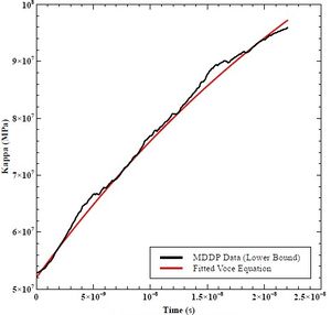
Figure 41: Fitted Voce Equation to Lower Bound MDDP Data.
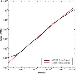
Figure 42: Fitted Voce Equation to Mean MDDP Data
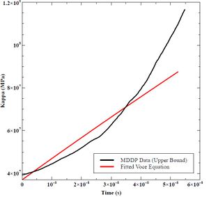
Figure 43: Fitted Voce Equation to Upper Bound MDDP Data
Table 9: K0, KS, and h0 Values for Lower Bound, Mean, and Upper Bound Mobility in MDDP.
| Parameter | Value |
|---|---|
| Lower Bound K0 (MPa) | 52 |
| Mean K0 (MPa) | 45 |
| Upper Bound K0 (MPa) | 37 |
| Lower Bound KS (MPa) | 150 |
| Mean KS (MPa) | 600 |
| Upper Bound KS (MPa) | 700 |
| Lower Bound h0 (GPa) | 27.5 |
| Mean h0 (GPa) | 25 |
| Upper Bound h0 (GPa) | 10 |
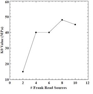
Figure 44: Initial strength (K0) value versus # of FRS in BCC chromium.
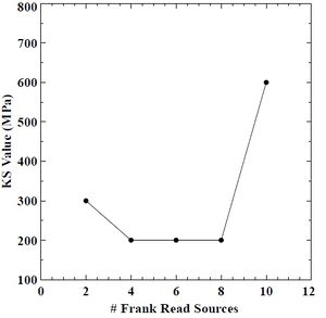
Figure 45: Saturation strength (Ks) value versus # of FRS in BCC chromium
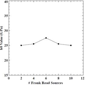
Figure 46: Hardening rate (h0) value versus # of FRS in BCC chromium
Crystal Plasticity
Single Crystal Stress Strain Behavior
The Voce hardening law material constants are upscaled to the mesoscale via MDDP computations using lower scale mobility information. We simulate hardening of Cr within a single Crystal Plasticity Finite Element Method (CPFEM) ABAQUS model. By understanding dislocation interaction at the microscale, we can determine hardening and plastic deformation at higher length scales. The mechanical response for each MEAM parameter set was nearly identical. Figure 47 depicts the stress-strain data provided from MDDP. Each MDDP calculation ran for 30 time steps. The plotted data shows mostly linear elastic response, but dislocations are present within the crystal.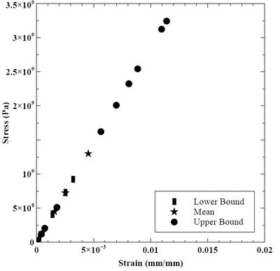
Figure 47. Stress-strain response in lower bound, mean, and upper bound
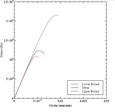
Figure 48. Stress-strain response from upper bound, mean, and lower bound dislocation dynamics simulation.
Polycrystal Stress Strain Behavior
In this section we used Abaqus to generate true stress-true strain curves from three different hardening laws for tension, compression, and torsion (simple shear) at a strain rate of roughly 1/s. Theses curves were generated for both a single crystal, single element simulations and a polycrystalline (500 grains), single element simulations. We used an elastic modulus of 210000 GPa and Poisson’s ratio of 0.30 for all the polycrystalline simulations and the single-crystal torsion simulations. Figure 49, Figure 50, and Figure 51 present the tension, compression, and torsion stress-strain curves, respectively. Tensile and compressive stress-strain curves are presented as axial stresses and strains, but torsional stress-strain curves are presented as Von Mises equivalent stresses and strains. Furthermore, the shear strain in the torsion (simple shear) simulations was assumed to be roughly equivalent to the Von Mises equivalent strain.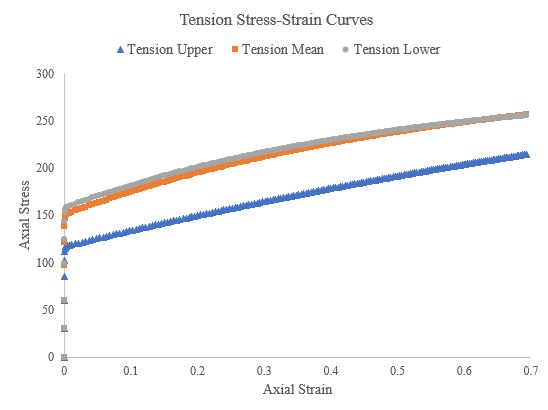
Figure 49.Tensile stress-strain curves of a 500 grain, single-element simulation for the upper, mean, and lower Voce hardening law parameters.
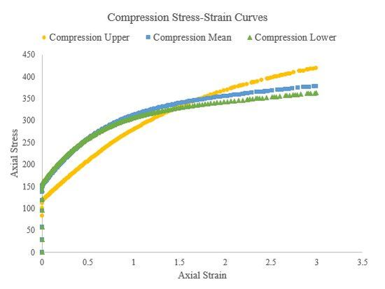
Figure 50.Compressive stress-strain curves of a 500 grain, single-element simulation for the upper, mean, and lower Voce hardening law parameters.
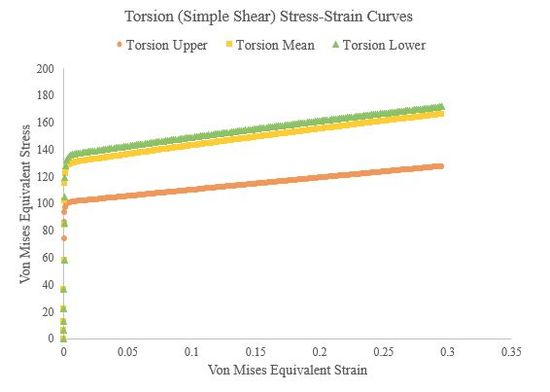
Figure 51.Torsion (simple shear) stress-strain curves of a 500 grain, single-element simulation for the upper, mean, and lower Voce hardening law parameters.

Figure 52.Tensile stress-strain curves of the 500 grain simulations and single grain simulations for the upper, mean, and lower Voce hardening law parameters.
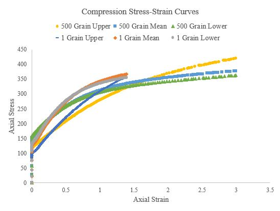
Figure 53.Compressive stress-strain curves of the 500 grain simulations and single grain simulations for the upper, mean, and lower Voce hardening law parameters.
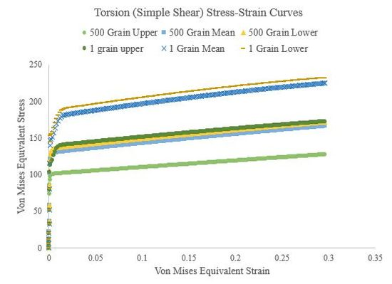
Figure 54.Torsional stress-strain curves of the 500 grain simulations and single grain simulations for the upper, mean, and lower Voce hardening law parameters.
Internal State Variable Model
Calibration
In this section we use the stress-strain behavior from the polycrystalline single element CPFEM to calibrate an ISV model with the DMGfit tool and then verify our results with another set of single element analysis in Abaqus. A tutorial for using the MSU DMGfit tool to calibrate an ISV model to experimental data can be found here. With the tool, we can find useful material constants for the ISV model that are used in a finite element calculation as a User Material subroutine (UMAT) in Abaqus. In this work, we fit three ISV models, one for the lower, mean, and upper sets of data we have been collecting. Ideally, the ISV model would capture temperature effects, strain rate dependencies, damage, hardening, and recovery for a range of loading conditions. However, in this work, we are limited to a single strain rate, a constant temperature, and disregard cyclic hardening/recovery and damage. Upon opening the DMGfit tool, we load in a set of tension, compression, and torsion data points and then list out our material dataset parameters. The only parameters we adjusted in the dataset are listed below in Table 10. The period was calculated automatically from the assigned strain rate.Table 10. ISV dataset input parameters
| Dataset Parameter | Value |
|---|---|
| Units | 5 = MPa |
| Strain Rate (1/s) | 1 |
| Tinit (initial temperature) | 300 K |
| G (Shear Modulus (MPa)) | 110000 |
| Bulk (Bulk Modulus (MPa)) | 251000 |
| Tmelt (melting temperature (K)) | 2180 |
Table 11. ISV material constants
| Material Constant | Lower ISV | Mean ISV | Upper ISV |
|---|---|---|---|
| Yield Stress (C3) | 158.52 | 148.98 | 115.22 |
| Transition (C5) | 1.036 | 1.036 | 1.036 |
| Kinematic anisotropic hardening (C9) | 0 | 0 | 127.78 |
| Kinematic dynamic recovery (C7) | 0.00217 | 0.00223 | 0.00223 |
| Isotropic hardening modulus (C15) | 227.95 | 264.91 | 66.85 |
| Isotropic dynamic recovery (C13) | 0.0034 | 0.0034 | 0.5146 |
Verification
To verify the ISV model calibration, we updated the input decks from the original polycrystalline CPFEM single element analysis with the new set of dependent variables and material constants. Additionally, to avoid hourglassing errors in the analysis, we changed the element type from C3D8R to a fully integrated C3D8 element. We submitted nine simulations to verify the three ISV models for tension, compression, and torsional loading. In Figures 55, 56, and 57, we show the overlaid stress-strain results for the original single element analysis, the ISV model fit, and the single element analysis with the ISV user material subroutine.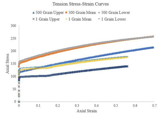
Figure 55.Mean Compression ISV model compared to the verification single element analysis and original.
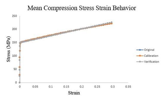
Figure 56.Mean Tension ISV model compared to the verification single element analysis and original.
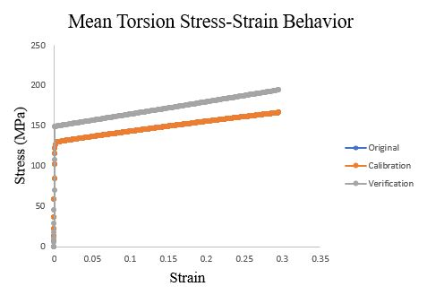
Figure 57.Mean Torsion ISV model compared to the verification single element analysis and original.
Theoretical Models
MEAM
We use atomistic analysis methods, suggested by Lee et al.[7], to describe the energy of a system related to interatomic forces and the relative position of atoms. According to the EAM developed by Baskes [8], the total energy of a system is composed of the embedding function Fi and pair interaction φ terms shown in Equation 3 below:where E is energy, ρi is background electron density, φ is atomic pair interaction, and Rij is distance. We describe the atomic pair interactions (φ) at a distance R in Equation 4 below:
where Z is the number of first neighbors, Eu (R) is the background electronic density, and ρ-0 (R) is energy per atom for the reference structure. We use the universal equation of state (UEOS) or first principles computations to obtain the atomic energy (Eu (R)). We calculate the UEOS parameters of cohesive energy (Ec), nearest neighbor distance (re), atomic volume (Ω), and bulk modulus (B) at equilibrium in the reference structure in Equations 5, 6, and 7, respectively.
The MEAM embedding function comprises the aforementioned terms and the adjustable parameter A as shown in Equation 8 below:
The background electron density is the combination of the spherically symmetric (ρ(0)) and angular (ρ(1), ρ(2), ρ(3)) partial electron density terms:
where the terms α, β, γ represent summations over the x, y, and z coordinate directions. Atomic electron density ρα(h) decreases exponentially with increasing distance ri between an atom i and the site of interest as illustrated in Equation 10 that contains constant decay lengths, βh.
The equations for the partial electron densities are coordinate invariant and equal to zero for cubic symmetric crystals. We represent the angular contributions from the partial electron densities in simplified form in Equation 10 (with constants th) and the equation for background electron density in Equation 11.
In order to obtain accurate material properties and avoid imaginary electron densities for Γ<-1, we use the functional form of G (shown in Equation 11) where G(0)=1/2. When G(0)=1, the background electron density is non angular dependent and is equivalent to the EAM expression for ρ[8].
Voce Law
We define the Voce law for materials exhibiting isotropic work-hardening or stress saturation at elevated stresses or strains in Equation 2 below. This equation represents how the flow stress evolves with plastic work.where κS is the saturation strength. The initial strength and hardening rate are given by &kapps;0 and h0, respectively. Moreover, the constant plastic shear strain rate, C, is computed with DD[3], [9].
Conclusions
In this work, we present DFT and MEAM simulations for pure chromium. We started by generating EA and EV curves and computing the bulk modulus, lattice parameter, and minimum cohesive energy. These values converged at 8 K point grid and energy cutoff of 60 Rydberg. A bulk modulus of 251 GPa, lattice parameter of 2.845 Å, and minimum cohesive energy of -4.10 eV was found for BCC chromium. DFT simulation data is in good agreement with existing literature. First principles computations were linked to atomistics through the calibration of MEAM model constants to DFT results and elastic moduli found in literature. Information obtained using atomistic methods is passed on to dislocation dynamics simulations at the microscale. To visualize dislocation movement within chromium, we produced a structure in LAMMPS with several atoms and a dislocation present. Once we had a converged system without too much image effects, we sheared the top and bottom rows of atoms and received dislocation position and time information. From those results, we calculated the dislocation velocity and calculated the mobility from three MEAM parameter sets. The stress-strain response and dislocation loop movement from MDDP gave us crucial information to feed a crystal plasticity model. After analyzing dislocation formation and movement within a crystal given a mechanical stimulus, we create our crystal plasticity model of Cr through hardening law development.References
- ↑Integrated Computational Materials Engineering (ICME) for Metals, 1st ed. John Wiley & Sons, Ltd, 2018. doi: 10.1002/9781119018377.
- ↑M. F. Horstemeyer et al., “Hierarchical Bridging Between Ab Initio and Atomistic Level Computations: Calibrating the Modified Embedded Atom Method (MEAM) Potential (Part A),” JOM, vol. 67, no. 1, pp. 143–147, Dec. 2014, doi: 10.1007/s11837-014-1244-0.
- ↑M. F. Horstemeyer, Integrated Computational Materials Engineering (ICME) for Metals: Using Multiscale Modeling to Invigorate Engineering Design with Science. Wiley, 2012. [Online]. Available: https://books.google.com/books?id=KCRLnYj1YiYC
- ↑J. Meija et al., “Atomic weights of the elements 2013 (IUPAC Technical Report),” Pure and Applied Chemistry, vol. 88, no. 3, pp. 265–291, Mar. 2016, doi: 10.1515/pac-2015-0305.
- ↑K. Yang, L. Lang, H. Deng, F. Gao, and W. Hu, “Modified analytic embedded atom method potential for chromium,” Modelling Simul. Mater. Sci. Eng., vol. 26, no. 6, p. 065001, Jun. 2018, doi: 10.1088/1361-651X/aaca48.
- ↑J. M. Hughes et al., “Hierarchical Bridging Between Ab Initio and Atomistic Level Computations: Sensitivity and Uncertainty Analysis for the Modified Embedded-Atom Method (MEAM) Potential (Part B),” JOM, vol. 67, no. 1, pp. 148–153, Dec. 2014, doi: 10.1007/s11837-014-1205-7.
- ↑B.-J. Lee, W.-S. Ko, H.-K. Kim, and E.-H. Kim, “The modified embedded-atom method interatomic potentials and recent progress in atomistic simulations,” Calphad, vol. 34, no. 4, pp. 510–522, Dec. 2010, doi: 10.1016/j.calphad.2010.10.007.
- ↑M. I. Baskes, “Determination of modified embedded atom method parameters for nickel,” Materials Chemistry and Physics, vol. 50, no. 2, pp. 152–158, Sep. 1997, doi: 10.1016/S0254-0584(97)80252-0.
- ↑D. P. Rao Palaparti, B. K. Choudhary, and T. Jayakumar, “Influence of Temperature on Tensile Stress–Strain and Work Hardening Behaviour of Forged Thick Section 9Cr–1Mo Ferritic Steel,” Trans Indian Inst Met, vol. 65, no. 5, pp. 413–423, Oct. 2012, doi: 10.1007/s12666-012-0146-5.